CGO 03-1: Colorization using Optimization
CGO 03-1: Colorization using Optimization
Homework
Please do the following steps and then upload the completed notebook to Moodle.
- Read the paper (yes it is very short)
- Answer in your own words how the formulation in the paper is converted to a least-squares optimization problem (you can look at the code, and please answer in the area provided below)
- Fill out the TODOs in the code and make sure the code works with the test image (result should look the same as in the paper)
- Try with another image (you can use other images from the paper)
Please check the deadline on Moodle.
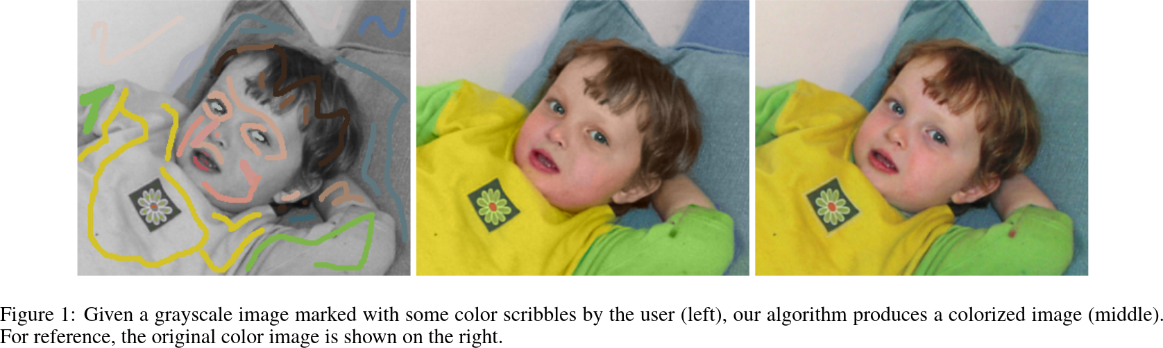
Colorization using Optimization
Colorization using Optimization Anat Levin, Dani Lischinski, Yair Weiss ACM Transactions on Graphics (SIGGRAPH), 2004
Useful links
Background
Digital images are made of discrete values known as pixels (comes from abbreviation of picture elements). These can be stored in many different colorspaces. For example, it is standard to encode pixels in RGB (Red-Blue-Green) colorspace, where each pixel is a $\mathbb{R}^3$ vector and each the three dimension corresponds to red, green, and blue. It is common to use other colorspaces such as YUV in which the luminance (greyscale) is encoded in a single channel, and the chrominance (colors) are encoded in to other channels. This is important in computer graphics as it lets us elegantly split different components of the image for further processing. Colorization using Optimization is an example of research that uses the YUV colorspace.
Approach
The approach is very simple and consists of minimizing the follow function in the YUV colorspace:
$ J(U) = \sum_r \left( U(r) - \sum_{s \in N(r)} w_{rs} U(s) \right)^2 $
where $U(r)$, $U(s)$ are the chrominance values of pixels $r$ and $s$, respectively, $N(r)$ is a neighbourhood of pixel $r$, and $w_{rs}$ is a weighting function that sums to one.
While there are many different possible weighting functions, the authors propose using the following one:
$ w_{rs} \propto \exp \left( \frac{-\left(Y(r)-Y(s)\right)^2}{2 \sigma_r^2} \right) $
where $Y(r)$ and $Y(s)$ are the luminance values of pixels $r$ and $s$, respectively, and $\sigma_r^2$ is the variance of the neighbourhood $N(r)$.
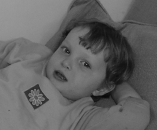
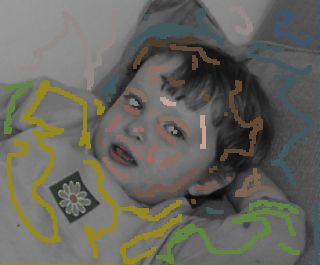
Test Images
You will need to download them and put them in the same directory as the notebook for them to work.
How to convert this into an optimization problem?
TODO Please answer how the formulation in the paper is converted to a least-squares optimization problem here. Why do we need a sparse matrix? You can use LaTeX to write mathematics. Japanese is also accepted.
Code
%matplotlib inline
import numpy as np
import matplotlib.pyplot as plt
from PIL import Image
from skimage import color
from scipy.sparse import csr_matrix
from scipy.sparse.linalg import spsolve
# Load the images
img_in = color.rgb2yuv( np.array( Image.open( 'baby.png' ).convert("RGB"), dtype=float ) / 255 )
img_edit = color.rgb2yuv( np.array( Image.open( 'baby_marked.png' ).convert("RGB"), dtype=float ) / 255 )
img_hint = np.zeros( img_edit.shape )
idx = (np.abs((img_in-img_edit).sum(2)) > 1e-4)
img_hint[ idx ] = img_edit[ idx ]# Show the input images and hints
fig = plt.figure()
fig.add_subplot(1,3,1).set_title('Input Image')
plt.imshow( color.yuv2rgb(img_in) )
fig.add_subplot(1,3,2).set_title('Hint Image')
plt.imshow( color.yuv2rgb(img_edit) )
fig.add_subplot(1,3,3).set_title('Color Hints')
plt.imshow( color.yuv2rgb(img_hint) )
plt.show()# Create the optimization problem
w = img_edit.shape[0]
h = img_edit.shape[1]
wpx = 1 # window size
b_u = np.zeros( (w*h,) )
b_v = b_u.copy()
# Sparse matrix
row = []
col = []
dat = []
for u in range(w):
for v in range(h):
i = v*w + u
# Add first entry U(r) for both channels
row.append( i )
col.append( i )
dat.append( 1. )
# Skip coloured areas
if idx[u,v]:
b_u[i] = img_edit[u,v,1]
b_v[i] = img_edit[u,v,2]
continue
umin = max(0,u-wpx)
umax = min(w,u+wpx+1)
vmin = max(0,v-wpx)
vmax = min(h,v+wpx+1)
patch = img_in[ umin:umax, vmin:vmax, 0 ]
mu_r = np.mean( patch )
sigma_r = np.var( patch )
sigma_r = max( sigma_r, 1e-6 )
Yr = img_in[u,v,0]
# Go over neighbours
N = []
wrs = []
for nu in range( umin, umax ):
for nv in range( vmin, vmax ):
j = nv*w + nu
if i==j:
continue
Ys = img_in[nu,nv,0]
# TODO Implement the weighting function
wrs.append( ... )
N.append(j)
wrs = np.array( wrs )
wrs /= wrs.sum()
for k,j in enumerate(N):
# TODO Finish creating the entries for the matrix
# Create sparse matrix
A = csr_matrix( (dat, (row,col)) )# Solve the optimization and display results
Y = img_in[:,:,0:1]
U = spsolve(A, b_u).reshape( h, w, 1 ).transpose( (1,0,2) )
V = spsolve(A, b_v).reshape( h, w, 1 ).transpose( (1,0,2) )
img_out = np.concatenate( (Y,U,V), axis=2 )
plt.imshow( color.yuv2rgb(img_out) )
plt.show()# Show the individual Y, U, and V channels
fig = plt.figure()
fig.add_subplot(1,3,1).set_title('Y')
plt.imshow( Y )
fig.add_subplot(1,3,2).set_title('U')
plt.imshow( U )
fig.add_subplot(1,3,3).set_title('V')
plt.imshow( V )
plt.show()